Linear Approximations and Differentials

Linear Approximations #

The motivation for this section is that we will want to be approximating a function near a point by their tangent lines at that point.

Sample (very) basic example: #

We’re going to approximate $f(x) = x^2$ around $x=2$.

1. Find the tangent line at $x=2$

   The derivative is $y = 2x$. The tangent line then is going to be: $\begin{align*} y-4 &= 4(x-2) \ y &= 4x - 4 \end{align*}$

2. Try to approximate (1.9)^2 using the tangent line:

   Since 1.9 is “close” to 2, we can use the tangent line at 2:

   $\begin{align*} y &= 4(1.9) - 4 \ &= 7.6 - 4 \ &= 3.6\end{align*}$

   Since the actual value $(1.9)^2 = 3.61$, that’s pretty close. Not bad!

3. What about approximating $(1)^2$?

   …. 1 is not “close” to 2.

   $\begin{align*} y &= 4(1) - 4 \ &= 0\end{align*}$

   and obviously $1^2 \ne 0$, so this is really crappy approximation.

Linear Approximations / Linearization #

In general, the tangent line to a function at the point $(a, f(a))$ is: $$ y - f(a) = f’(a) (x-a) $$

We’ll solve for $y$, label it $L(x)$, and give it the name linearization: $$ L(x) = f(a) + f’(a)(x-a) $$

Note This is called linearization, a linear approximation, or the first-order Taylor Polynomial¹ for $f$ at $x=a$.

Example #

Approximate $y=\sin(x)$ for $x$ values near 0.

Since $$ f(x) \approx f(a) + f’(a) (x-a) $$

Find $a, f(a), f’(x),$ and $f’(a)$ to find the linear approximation.

Give it a try before revealing the solution here:

Now let’s use the approximation to approximate $\sin(1^\circ)$.

Example #

1. Find the linearization of $\sqrt[5]{32-4x}$ around $x=0$.
2. Use that linearization to approximate $\sqrt{27.99}$

Example: #

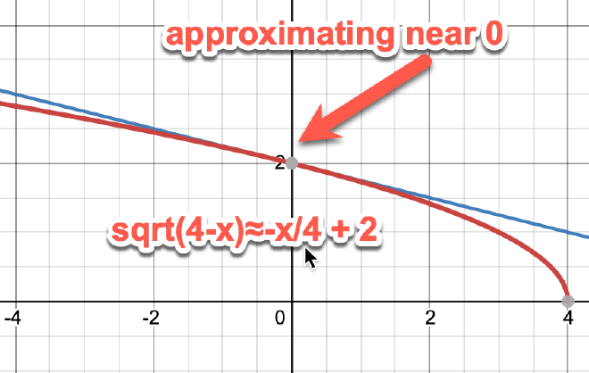
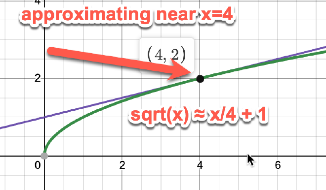
Evaluating $\sqrt{3.99}$ in two ways, once, centering on $x=0$, and second, centering on $x=4$:

To approximate around $x=0$, we need the function that you’re using to approximate to be sqrt(4-x):

Here’s using the given function: #

and in order to get $\sqrt{3.99}$, you need to plug in $x=0.01$.

On the other hand, here’s using the function $\sqrt{x}$ around x=4. Notice that you’ll still get the same answers, but the $x$ values you’re using are very different

here to approximate $\sqrt{3.99}$ you need to plug in $x=3.99$.

Differentials #

Recall that $f’(x) = \dfrac{\text{ change in y’s }}{\text{change in x’s}}$

so $f’(x) \approx \dfrac{\Delta y}{\Delta x}$ and let $\Delta x \to 0$, we get Leibniz notation:

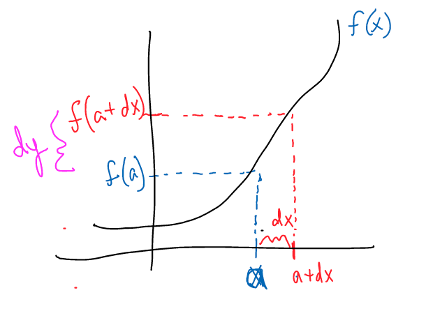
$$ f’(x) = \dfrac{dy}{dx} $$ and solving for $dy$ we get the differentials $$ dy = f’(x) dx $$

This defines the differential $dy$ in terms of the variables $x$ and $dx$.

Example #

If $f(x) = \sqrt{x+1}$, find $dy$.

Solution: (try it before revealing the spoiler)

Connection of differentials to linear approximations #

$$ f(a + dx) \approx f(a) + dy $$ a tiny, tiny change in $dx$ changes the function by the tiny, tiny change $dy$.

For concrete (less tiny) changes, we’ll write $\Delta x$ and $\Delta y$ to have:

$$ f(a + \Delta x) \approx f(a) + \Delta y $$

Example #

For example, using $f(x) = \sqrt{x+1}$, let $a=3$ and $\Delta x = 0.1$, find the approximation of $\sqrt{4.1}$

Solution: set up $$ \begin{align*} f(3 + \Delta x) &= f(3+0.1) \ &= f(3.1) \ &= \sqrt{3.1+1} \end{align*} $$ so $$ \begin{align*} f(3+\Delta x) = \sqrt{4.1} &\approx f(3) + \Delta y \ &\approx f(3) + \dfrac{\Delta x}{2\sqrt{3+1}} \ &= \sqrt{3+1} + \dfrac{0.1}{2\sqrt{3+1}} \ &= 2 + \dfrac{0.1}{4} \ &= 2.025 \end{align*} $$

… note that the calculator says $\sqrt{4.1} \approx 2.02484$, so we’re pretty close!